A Peek into a Quantum Computer
Examples of quantum error correction in an IBM Quantum device.

I did some livestreams on YouTube at the end of last year. Their purpose was to spread the Christmassy joy of quantum error correction. Here they are if you are interested.
In my opinion, the best part was when I took data from real quantum computers and visualized them in the second video. I was using the same Jupyter notebook today, and thought I’d produce some more of those images and dump them in a blog post. This blog post, in fact! The image at the top of the page is the first example.
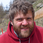
These images represent the decoding graph for d=9 repetition codes run for T=9 syndrome measurement round on the IBM Quantum device ibm_geneva. The red nodes represent events at which a signature of an error were detected. The blue ones are where everything is fine. We don’t know about the yellow ones, since measuring those would disturb our stored information. Each image represents a different run, and a different set of errors.
When the errors occur on the qubits that store information, they cause a pair of nodes that are separated by a horizontal or diagonal line. When there is a failure in the measurements made during the process, the pairs are separated vertically. The image above therefore suggests that a particular measurement failed twice in a row.
In the following images you’ll see examples of increasing amounts of noise. The first image is an example of a run in which at least 15 red nodes were found, and the last has at least 27.
You might notice that the first ones look like they are made of a lot of vertically separated pairs. The last ones are more complex, and are probably a mix of both horizontal and vertical errors. This is due to the fact that measurement errors are much more likely than any others in IBM Quantum systems.